Deep Autoencoder - Kotlin
I recently decided to make the switch from Java to Kotlin, that switch included the urge to reprogram a bunch of neural network stuff.
Code can all be found on GitHub: here
The codebase originally started as a simple autoencoder trained via backpropagation. I then extended this to support a stacked (deep) architecture as well as convolution. The premise of an autoencoder is really quite straight forward once you've grasped the basics of a single feed-forward neural network.
The vanilla autoencoder can be thought of as two single-layer neural networks stacked together. The first neural network is commonly referred to as the "encoder" network, and the second network called the "decoder". Given training data %%x%%, the encoder network will have input size of %%|x|%% and an output size of %%|h|%%, and the decoder network will have input size of %%|h|%% and output size of %%|x|%%.
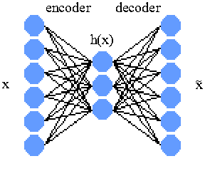
Typically %%|h|%% is smaller than %%|x|%% as this has the effect of forcing the neural network to find a way to represent the input data using less bits of information. This bottle necking results in compression, feature clustering, dimension reduction, etc., all of which are some properties of learning. There are also advantages in expanding middle layers in networks but that is outside the scope of this demo.
The training process is to propagate the training data, %%x%% sequentially through the encoder and decoder networks. The target, or training data of the final output is the original training data %%x%%. In other words the autoencoder learns by trying to "learn itself".
To stack autoencoders to form a deep autoencoder you first create another autoencoder, and it's job is to learn the encoded feature (output of the encoder network, %%|h|%%). You can repeat this process as much as you like with a wide variety of possible configurations.
Supported Neural Networks
- Autoencoder
- Stacked (Deep) Autoencoder
- Stacked (Deep) Convolution Autoencoder
- Feature Clustering via Autoencoder
- Error Backpropagation Multi-Layer Perceptron
- Continuous Webcam Learning w/ Deep Autoencoder
Training Algorithms
- Stochastic Gradient Descent
- Mini-batch size = 1
MNIST Training Results
Single Layer Autoencoder
Training Rate: 0.05 Steps: 1,000,000 Algorithm: Stochastic Gradient Descent Error: ~2.6 (Squared error of pixel error per image, training data)


Click image to see all 60,000k reconstructions. (Good results can be seen in far less than 1,000,000 steps.)
Deep Autoencoder
Training Rate: 0.1 Steps: 250,000 Algorithm: Stochastic Gradient Descent Error: ~5.6 (Squared error of pixel error per image, training data)

Click image to see all 60,000k reconstructions.
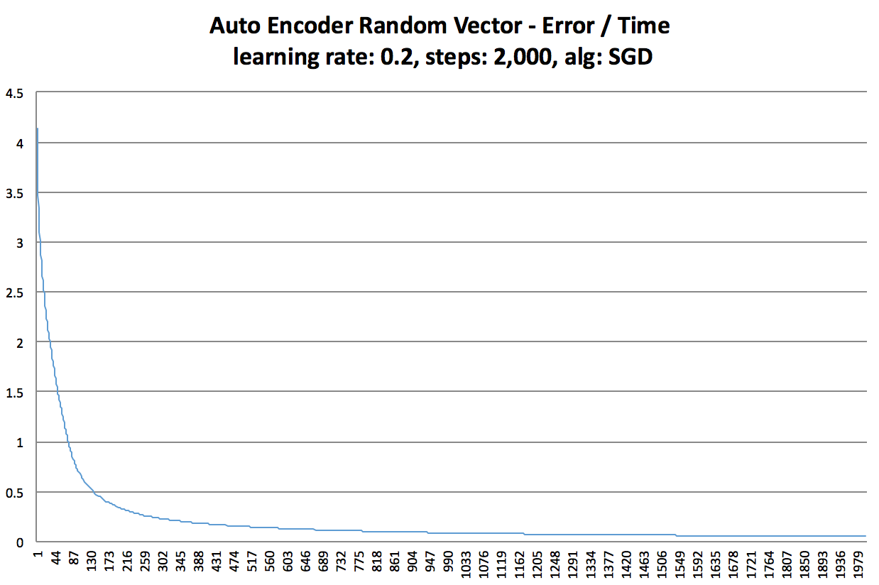
Random Vectors
Below are a few error graphs of a single layer autoencoder learning random vectors.
Feature Clustering
A byproduct of an autoencoder learning to encode features, is that through the encoding/compression process, feature clustering also occurs.
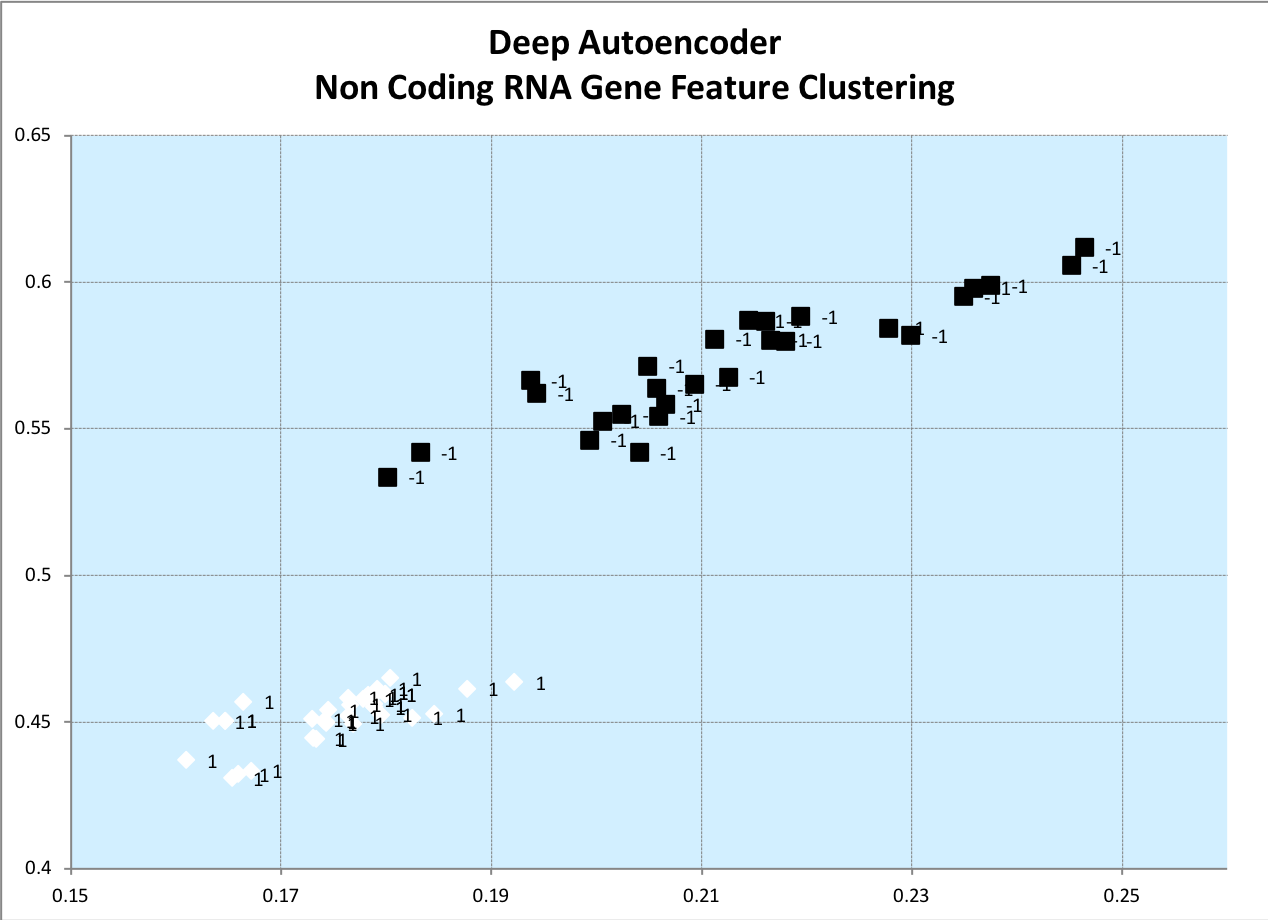
Below are examples of a deep autoencoder learning to encode input vectors. The deepest most layer maps to a small 2-dimensional feature vector so that we can easily visualize the encoding on a x-y plot.
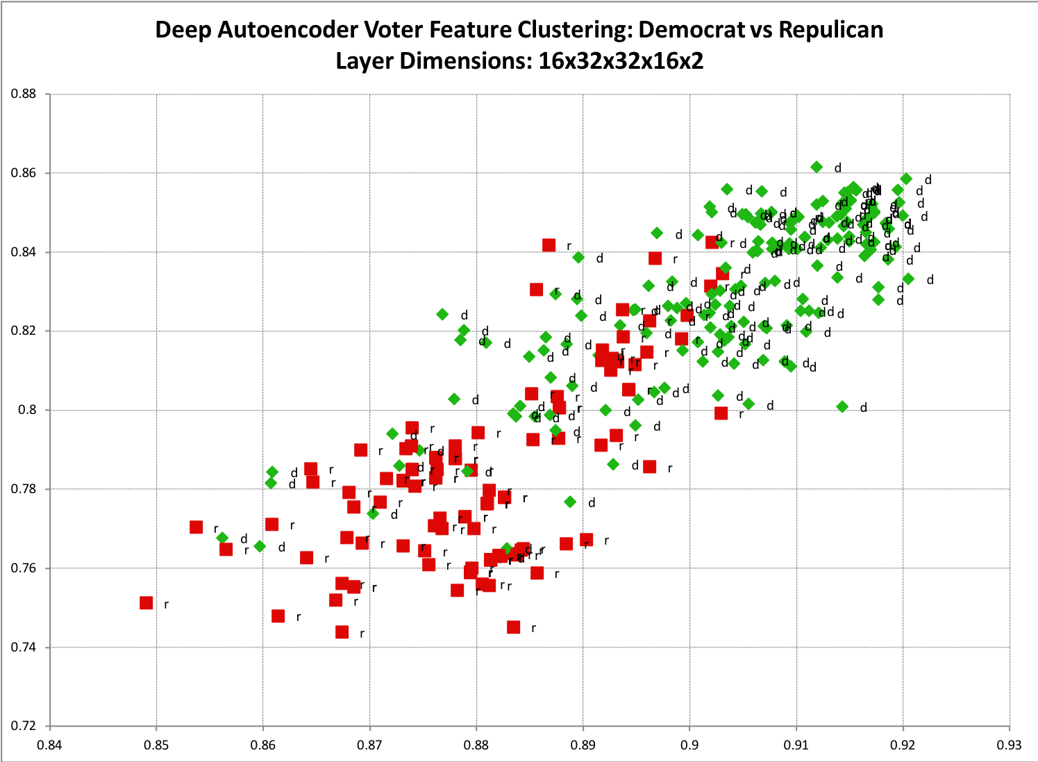
Republican and Democrat Voting History Clustering
The deepest most layer maps to a small 2-dimensional feature vector so that we can easily visualize the encoding on a x-y plot. There is a clear trend showing democratic votes clustered to the top right, and republican to the bottom left. Unsurprisingly, there is also some overlap demonstrating cases where democrats and republicans share overlapping votes.
Non-Coding RNA Gene Clustering
Deep Convolutional Autoencoder
Vanila Autoencoders work great for low dimensional data. However, high dimensional data, such as images require a few tricks to effectively train. By using a single autoencoder with a single fully-connected encode/decode weight matrix, we are effectively saying that every single pixel is directly correlated to every other pixel. While this may be true, the relation of pixels of opposite corners, or large distances apart in an image are likely more abstractly related. Asking a neural network to encode that many correlations in a single layer is a very steep request. You may also discover that the weight matrices are too large to fit in memory, or too costly to compute. A solution to this is to break each layer into pieces and train smaller networks on subsections of the image. The separate networks are then connected together in subsequent layers. This allows the network to learn simpler features first before combining in other layers to form more abstract features. The idea is that pixels closer to each other are likely more immediately related to each other. Additionally, it helps that this also results in smaller matrices which means faster computation and potential parellization. Note that extra work was done to ensure spatial relations when processing 2d data is preserved when splitting/merging data between convolution layers.
Learning of a single small image
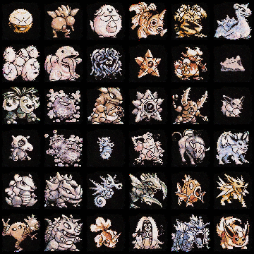
Learning a batch of Pokemon Images
This may just be an illusion, but I find it interesting that the network appears to be learning the shape and structure before color. Note, I'm using a small network and a low number of training cycles. With more training this image will become more clear.

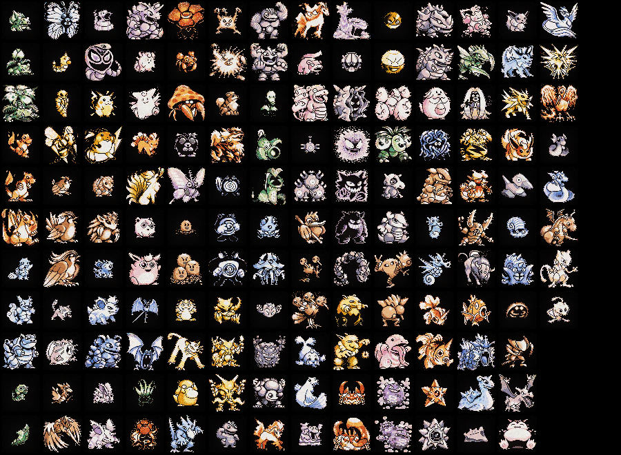
Learning all 151 pokemon images
Note that the color model hasn't been fully learned. Also there are some strange clipping/white spots. These are largely due to editing issues with the training image on my part. :)

Webcam Learning
The next fun thing to do with an Autoencoder is to hook it up to your webcam and have it watch and learn you and your sorroundings. Code found here
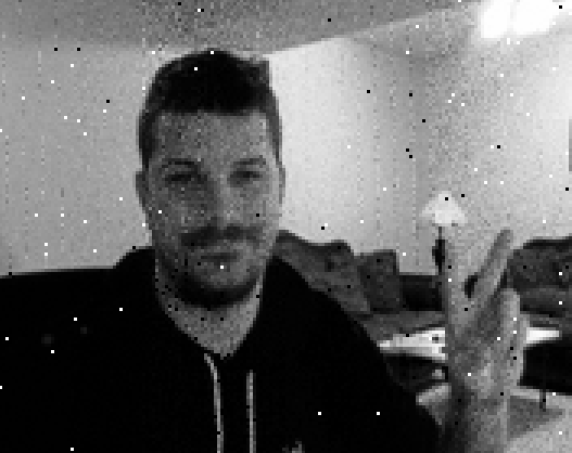
Three videos showing the first steps of webcam learning.
- grayscale part 1: https://v.usetapes.com/LYwFNwMYln
- grayscale part 2: https://v.usetapes.com/wjRufz5gA2
- color part 1: https://v.usetapes.com/wjRufz5gA2
Error Backpropagation Multi-Layer Perceptron
Included is an implementation of a vanilla Multi-Layer Percepttron trained via Error Backpropagation. This network can be used in isolation or chained to the end of an autoencoder (or other network) to learn/interpret features.
XOR
layer sizes [2, 10, 1]
trained in 331ms
[0.000000, 0.000000] -> [0.047964]
[0.000000, 1.000000] -> [0.959066]
[1.000000, 0.000000] -> [0.960735]
[1.000000, 1.000000] -> [0.042386]
total error: 0.042637016544833546
Random Vectors
layer sizes [10, 15, 20, 10, 2]
trained in 870ms
870ms
[0.699696, 0.994488, 0.404887, 0.984956, 0.689970, 0.056813, 0.831808, 0.749085, 0.711832, 0.055555] -> [0.118158, 0.492797]
[0.925863, 0.689105, 0.915446, 0.001710, 0.107525, 0.824539, 0.525365, 0.658552, 0.229297, 0.361060] -> [0.895759, 0.552127]
[0.166542, 0.318311, 0.867185, 0.985580, 0.103086, 0.939888, 0.457910, 0.758986, 0.485288, 0.241934] -> [0.957250, 0.744716]
[0.287445, 0.069872, 0.958304, 0.072877, 0.660907, 0.079100, 0.689686, 0.049298, 0.130067, 0.314979] -> [0.699894, 0.362934]
[0.515721, 0.321559, 0.704876, 0.835021, 0.622173, 0.473566, 0.077452, 0.868374, 0.987843, 0.153353] -> [0.269416, 0.366104]
total error: 0.012446605931539503
MNIST Digits
Layer Sizes: [784, 300, 10], Learning Rate: 0.15, Algorithm: Stochastic Gradient Descent
train errors: 673
train error %: 1.1216666549444199%
train accuracy %: 98.87833334505558%
test errors: 259
test error %: 2.590000070631504%
test accuracy %: 97.4099999293685%
Misc Features
- Convoluted Layers can be configured to run in parallel.
Notes
-
Since SGD, mini batch = 1, is noisy, the error signal will spike up and down wildly as it converages. A trick I employ is to take the raw errors and group them into batches and compute the average errors after the fact.
awk '{sum+=%%1} (NR%10)==0{print sum/10; sum=0;}' /tmp/raw_errors.log > /tmp/avg_erros.logYou can also batch up groups and average in code. -
Converting everything from Double to Float was an instant 1.5x speedup. I don't suspect the GPU is actually being used and that is a pure Java speedup.
-
To run unit tests, run
mvn test(This will take a few minutes). -
Note that files ending in Demo.kt may have @Test annotations, they are to conveniently launch the programs and not part of the unit test suite.
 Arrived
 Ninja Turdle
 Twitch